7.1. Silicon
Silicon. 2x2x2 conventional supercell
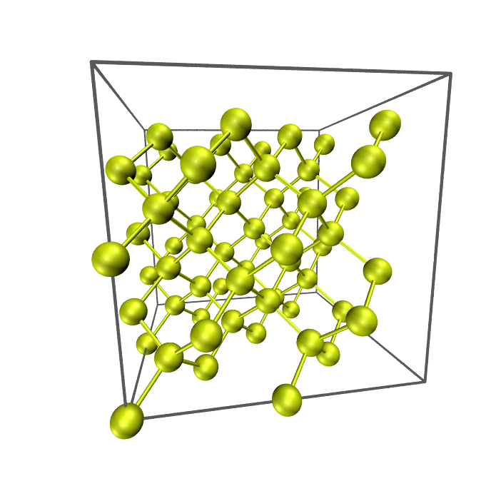
In the following, (anharmonic) phonon properties of bulk silicon (Si) are calculated by a 2x2x2 conventional cell containing 64 atoms.
1. Get displacement patterns by alm
Change directory to example/Si and open file si_alm.in. This file is an input for the code alm which estimate interatomic force constants (IFC) by least square fitting. In the file, the crystal structure of a 2x2x2 conventional supercell of Si is specified in the &cell and the &position fields as the following:
&general
  PREFIX = si222
  MODE = suggest
  NAT = 64; NKD = 1
  KD = Si
/

&interaction
  NORDER = 1  # 1: harmonic, 2: cubic, ..
/

&cell
  20.406 # factor in Bohr unit
  1.0 0.0 0.0 # a1
  0.0 1.0 0.0 # a2
  0.0 0.0 1.0 # a3
/

&cutoff
  Si-Si None
/

&position
  1 0.0000000000000000 0.0000000000000000 0.0000000000000000
  1 0.0000000000000000 0.0000000000000000 0.5000000000000000
  1 0.0000000000000000 0.2500000000000000 0.2500000000000000
  1 0.0000000000000000 0.2500000000000000 0.7500000000000000
  1 0.0000000000000000 0.5000000000000000 0.0000000000000000
  1 0.0000000000000000 0.5000000000000000 0.5000000000000000
  1 0.0000000000000000 0.7500000000000000 0.2500000000000000
Replace the lattice constant of the supercell (20.406 Bohr) by your own value.
Then, execute alm
$ alm si_alm.in > si_alm.log1
which creates a file si222.pattern_HARMONIC in the working directory. In the pattern file, suggested displacement patterns are defined in Cartesian coordinates. As you can see in the file, there is only one displacement pattern for harmonic IFCs of bulk Si.
2. Calculate atomic forces for the displaced configurations
Next, calculate atomic forces for all the displaced configurations defined in si222.pattern_HARMONIC. To do so, you first need to decide the magnitude of displacements \(\Delta u\), which should be small so that anharmonic contributions are negligible. In most cases, \(\Delta u \sim 0.01\) Å is a reasonable choice.
Then, prepare input files necessary to run an external DFT code for each configuration. Since this procedure is a little tiresome, we provide a subsidiary Python script for VASP, Quantum-ESPRESSO (QE), and xTAPP. Using the script displace.py in the tools/ directory, you can generate the necessary input files as follows:
QE
$ python displace.py --QE=si222.pw.in --mag=0.01 -pf si222.pattern_HARMONICVASP
$ python displace.py --VASP=POSCAR.orig --mag=0.01 -pf si222.pattern_HARMONICxTAPP
$ python displace.py --xTAPP=si222.cg --mag=0.01 -pf si222.pattern_HARMONICOpenMX
$ python displace.py --OpenMX=si222.dat --mag=0.01 -pf si222.pattern_HARMONIC
The --mag option specifies the displacement length in units of Angstrom.
You need to specify an input file with equilibrium atomic positions either by the --QE, --VASP, --xTAPP, --OpenMX or --LAMMPS.
Then, calculate atomic forces for all the configurations. This can be done with a simple shell script as follows:
#!/bin/bash

# Assume we have 20 displaced configurations for QE [disp01.pw.in,..., disp20.pw.in].

for ((i=1;i<=20;i++))
do
    num=`echo $i | awk '{printf("%02d",$1)}'`
    mkdir ${num}
    cd ${num}
    cp ../disp${num}.pw.in .
    pw.x < disp${num}.pw.in > disp${num}.pw.out
    cd ../
done
Important
In QE, you need to set tprnfor=.true. to print out atomic forces.
The next step is to collect the displacement data and force data by the Python script extract.py (also in the tools/ directory). This script can extract atomic displacements, atomic forces, and total energies from multiple output files as follows:
QE
$ python extract.py --QE=si222.pw.in *.pw.out > DFSET_harmonicVASP
$ python extract.py --VASP=POSCAR.orig vasprun*.xml > DFSET_harmonicxTAPP
$ python extract.py --xTAPP=si222.cg *.str > DFSET_harmonicOpenMX
$ python extract.py --OpenMX=si222.dat *.out > DFSET_harmonic
In the above examples, atomic displacements and corresponding atomic forces of all the configurations are merged as DFSET_harmonic.
These files will be used in the following fitting procedure as DFSET (See Format of DFSET).
Note
For your convenience, we provide the DFSET_harmonic file in the reference/ subdirectory. These files are generated by the Quantum-ESPRESSO package with --mag=0.02. You can proceed to the next step by copying these files to the working directory.
3. Estimate force constants by fitting
Edit the file si_alm.in to perform least-square fitting.
Change the MODE = suggest to MODE = optimize as follows:
&general
  PREFIX = si222
  MODE = optimize   # <-- here
  NAT = 64; NKD = 1
  KD = Si
/
Also, add the &optimize field as:
&optimize
  DFSET = DFSET_harmonic
/
Then, execute alm again
$ alm si_alm.in > si_alm.log2
This time alm extract harmonic IFCs from the given displacement-force data set (DFSET_harmonic).
You can find files si222.fcs and si222.xml in the working directory. The file si222.fcs contains all IFCs in Rydberg atomic units. You can find symmetrically irreducible sets of IFCs in the first part as:
 *********************** Force Constants (FCs) ***********************
 *        Force constants are printed in Rydberg atomic units.       *
 *        FC2: Ry/a0^2     FC3: Ry/a0^3     FC4: Ry/a0^4   etc.      *
 *        FC?: Ry/a0^?     a0 = Bohr radius                          *
 *                                                                   *
 *        The value shown in the last column is the distance         *
 *        between the most distant atomic pairs.                     *
 *********************************************************************

 ----------------------------------------------------------------------
      Index              FCs         P        Pairs     Distance [Bohr]
 (Global, Local)              (Multiplicity)
 ----------------------------------------------------------------------

  *FC2
       1       1     2.7613553e-01   1     1x     1x       0.000
       2       2    -9.5252308e-04   2     1x     2x      10.203
       3       3    -3.7574247e-04   2     1x    33x      10.203
       4       4     8.8561868e-03   1     1x     3x       7.215
       5       5     1.9633030e-03   1     1x     3y       7.215
       6       6    -3.9798276e-03   1     1x    17x       7.215
       7       7    -3.9080855e-03   1     1x    17z       7.215
       8       8     8.2188178e-03   4     1x     6x      14.429
       9       9     4.3878651e-05   4     1x    34x      14.429
      10      10    -6.7358757e-02   1     1x     9x       4.418
      11      11    -4.7360832e-02   1     1x     9y       4.418
      12      12     1.0670028e-03   1     1x    10x       8.460
      13      13    -8.2098635e-04   1     1x    10y       8.460
      14      14    -6.9742830e-04   1     1x    10z       8.460
      15      15     2.1135669e-04   1     1x    26x       8.460
      16      16    -4.3031422e-03   1     1x    11x      11.118
      17      17     5.0759340e-04   1     1x    11y      11.118
      18      18    -4.7178438e-04   1     1x    25x      11.118
      19      19    -4.7518256e-04   1     1x    25z      11.118
      20      20    -7.4138963e-04   2     1x    20x      12.496
      21      21     1.2900836e-03   2     1x    20y      12.496
      22      22    -1.7263732e-04   2     1x    20z      12.496
      23      23     6.4515756e-05   2     1x    35x      12.496
      24      24     3.5369980e-04   1     1x    28x      13.254
      25      25    -5.1486930e-04   1     1x    28y      13.254
Harmonic IFCs \(\Phi_{\mu\nu}(i,j)\) in the supercell are given in the third column and the multiplicity \(P\) is the number of times each interaction \((i, j)\) occurs within the given cutoff radius. For example, \(P = 2\) for the pair \((1x, 2x)\) because the distance \(r_{1,2}\) is exactly the same as the distance \(r_{1,2'}\) where the atom 2’ is a neighboring image of atom 2 under the periodic boundary condition. If you compare the magnitude of IFCs, the values in the third column should be divided by \(P\).
In the log file si_alm.log2, the fitting error is printed. Try
$ grep "Fitting error" si_alm.log2
Fitting error (%) : 0.567187
The other file si222.xml contains crystal structure, symmetry, IFCs, and all other information necessary for subsequent phonon calculations.
4. Calculate phonon dispersion and phonon DOS
Open the file si_phband.in and edit it for your system.
&general
  PREFIX = si222
  MODE   = phonons
  FCSXML = si222.xml

  NKD = 1; KD = Si
  MASS = 28.0855
/

&cell
  10.203
  0.0 0.5 0.5
  0.5 0.0 0.5
  0.5 0.5 0.0
/

&kpoint
  1  # KPMODE = 1: line mode
  G 0.0 0.0 0.0 X 0.5 0.5 0.0 51
  X 0.5 0.5 1.0 G 0.0 0.0 0.0 51
  G 0.0 0.0 0.0 L 0.5 0.5 0.5 51
/
Please specify the XML file you obtained in step 3 by the FCSXML-tag as above.
In the &cell-field, you need to define the lattice vector of a primitive cell.
In phonon dispersion calculations, the first entry in the &kpoint-field should be 1 (KPMODE = 1).
Then, execute anphon
$ anphon si_phband.in > si_phband.log
which creates a file si222.bands in the working directory. In this file, phonon frequencies along the given reciprocal path are printed in units of cm-1 as:
#  G X G L
# 0.000000 0.615817 1.486715 2.020028
# k-axis, Eigenvalues [cm^-1]
0.000000   1.097373e-10   1.097373e-10   1.097373e-10   5.129224e+02   5.129224e+02   5.129224e+02
0.012316   6.009520e+00   6.009520e+00   1.022526e+01   5.128286e+02   5.128286e+02   5.128923e+02
0.024633   1.200989e+01   1.200989e+01   2.044420e+01   5.125479e+02   5.125479e+02   5.128019e+02
0.036949   1.799191e+01   1.799191e+01   3.065053e+01   5.120824e+02   5.120824e+02   5.126510e+02
0.049265   2.394626e+01   2.394626e+01   4.083799e+01   5.114353e+02   5.114353e+02   5.124391e+02
0.061582   2.986346e+01   2.986346e+01   5.100034e+01   5.106114e+02   5.106114e+02   5.121656e+02
0.073898   3.573381e+01   3.573381e+01   6.113142e+01   5.096167e+02   5.096167e+02   5.118299e+02
You can plot the phonon dispersion relation with gnuplot or any other plot software.
For visualizing phonon dispersion relations, we provide a Python script plotband.py in the tools/ directory (Matplotlib is required.). Try
$ python plotband.py si222.bands
Then, the phonon dispersion is displayed as follows:
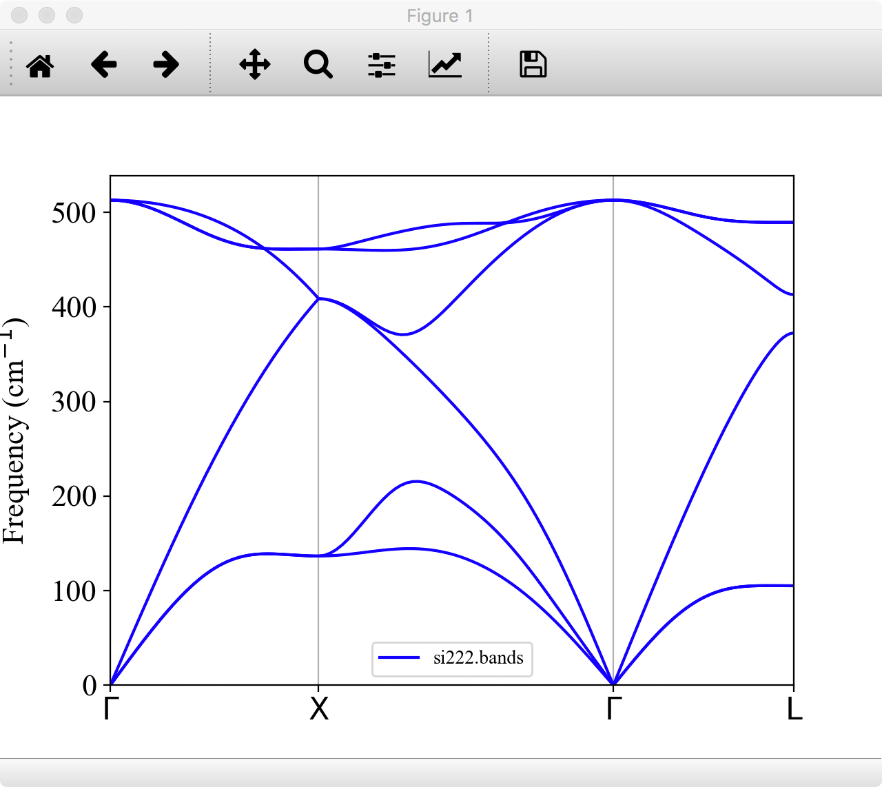
You can save the figure as png, eps, or other formats from this window.
You can also change the energy unit of phonon frequency from cm-1 to THz or meV by the --unit option.
For more detail of the usage of plotband.py, type
$ python plotband.py -h
Next, let us calculate the phonon DOS. Copy si_phband.in to si_phdos.in and edit the &kpoint field as follows:
&kpoint
  2  # KPMODE = 2: uniform mesh mode
  20 20 20
/
Then, execute anphon
$ anphon si_phdos.in > si_phdos.log
This time, anphon creates files si222.dos and si222.thermo in the working directory, which contain phonon DOS and thermodynamic functions, respectively. For visualizing phonon DOS and projected DOSs, we provide a Python script plotdos.py in the tools/ directory (Matplotlib is required.). The command
$ python plotdos.py --emax 550 --nokey si222.dos
will show the phonon DOS of Si by a pop-up window:
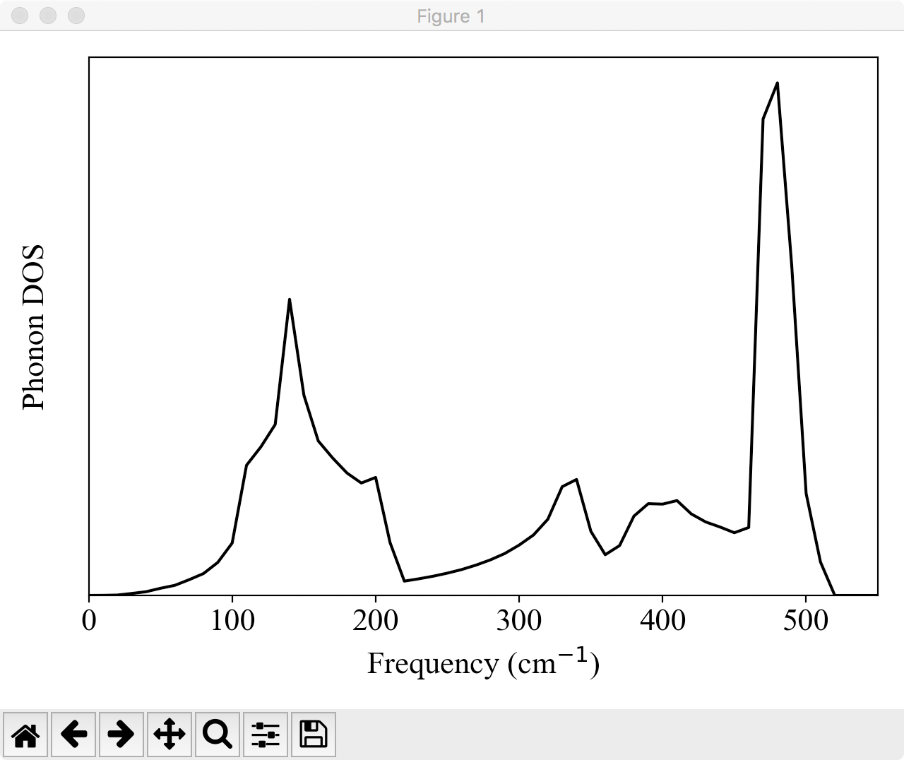
To improve the resolution of DOS, try again with a denser \(k\) grid and a smaller DELTA_E value.
5. Estimate cubic IFCs for thermal conductivity
Note
Note that there are more efficient ways to calculate anharmonic IFCs, especially when you calculate the quartic or higher-order terms. Please Tutorial 7.5 and Tutorial 7.6 for details.
Copy file si_alm.in to si_alm2.in. Edit the &general, &interaction, and &cutoff fields of si_alm2.in as the following:
&general
  PREFIX = si222_cubic
  MODE = suggest
  NAT = 64; NKD = 1
  KD = Si
/
Change the PREFIX from si222 to si222_cubic and set MODE to suggest.
&interaction
  NORDER = 2
/
Change the NORDER tag from NORDER = 1 to NORDER = 2 to include cubic IFCs.
Here, we consider cubic interaction pairs up to second nearest neighbors by specifying the cutoff radii as:
&cutoff
  Si-Si None 7.3
/
7.3 Bohr is slightly larger than the distance of second nearest neighbors (7.21461 Bohr). Change the cutoff value appropriately for your own case. (Atomic distance can be found in the file si_alm.log.)
Then, execute alm
$ alm si_alm2.in > si_alm2.log
which creates files si222_cubic.pattern_HARMONIC and si222_cubic.pattern_ANHARM3.
Then, calculate atomic forces of displaced configurations given in the file si222_cubic.pattern_ANHARM3, and collect the displacement and force datasets to a file DFSET_cubic as you did for harmonic IFCs in Steps 3 and 4.
Note
Since making DFSET_cubic requires moderate computational resources, you can skip this procedure by copying file reference/DFSET_cubic to the working directory. The file we provide is generated by the Quantum-ESPRESSO package with --mag=0.04.
In si_alm2.in, change MODE = suggest to MODE = optimize and add the following:
&optimize
  DFSET = DFSET_cubic
  FC2XML = si222.xml # Fix harmonic IFCs
/
By the FC2XML tag, harmonic IFCs are fixed to the values in si222.xml.
Then, execute alm again
$ alm si_alm2.in > si_alm2.log2
which creates files si222_cubic.fcs and si222_cubic.xml. This time cubic IFCs are also included in these files.
Note
In the above example, we obtained cubic IFCs by least square fitting with harmonic IFCs being fixed to the value of the previous harmonic calculation. You can also estimate both harmonic and cubic IFCs simultaneously instead. To do this, merge DFSET_harmonic and DFSET_cubic as
$ cat DFSET_harmonic DFSET_cubic > DFSET_merged
and change the &optimize field as the following:
&optimize
  DFSET = DFSET_merged
/
6. Calculate thermal conductivity
Copy file si_phdos.in to si_RTA.in and edit the MODE and FCSXML tags as follows:
&general
  PREFIX = si222
  MODE = RTA
  FCSXML = si222_cubic.xml

  NKD = 1; KD = Si
  MASS = 28.0855
/
In addition, change the \(k\) grid density as:
&kpoint
  2
  10 10 10
/
Then, execute anphon as a background job
$ anphon si_RTA.in > si_RTA.log &
Please be patient. This can take a while. When the job finishes, you can find a file si222.kl in which the lattice thermal conductivity is saved. You can plot this file using gnuplot (or any other plotting softwares) as follows:
$ gnuplot
gnuplot> set logscale xy
gnuplot> set xlabel "Temperature (K)"
gnuplot> set ylabel "Lattice thermal conductivity (W/mK)"
gnuplot> plot "si222.kl" usi 1:2 w lp
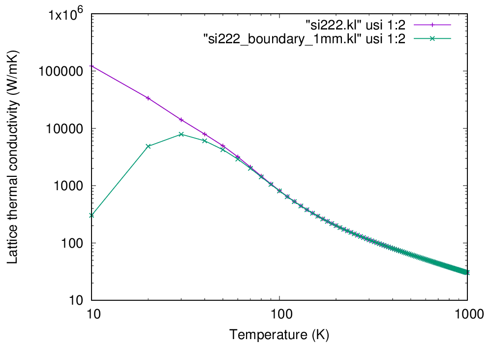
Calculated lattice thermal conductivity of Si (click to enlarge)
As you can see, the thermal conductivity diverges in \(T\rightarrow 0\) limit.
This occurs because we only considered intrinsic phonon-phonon scatterings in the present calculation and
neglected phonon-boundary scatterings which are dominant in the low-temperature range.
The effect of the boundary scattering can be included using the python script analyze_phonons.py in the tools directory:
$ analyze_phonons.py --calc kappa_boundary --size 1.0e+6 si222.result > si222_boundary_1mm.kl
In this script, the phonon lifetimes are altered using the Matthiessen’s rule
Here, the first term on the right-hand side of the equation is the scattering rate due to
the phonon-phonon scattering and the second term is the scattering rate due to a grain boundary of size \(L\).
The size \(L\) must be specified using the --size option in units of nm. The result is also shown in the
above figure and the divergence is cured with the boundary effect.
Note
When a calculation is performed with a smearing method (ISMEAR=0 or 1) instead of the
tetrahedron method (ISMEAR=-1), the thermal conductivity may have a peak structure in the very low-temperature region even without the boundary effect. This peak occurs because of the finite smearing width \(\epsilon\) used in the smearing methods. As we decrease the \(\epsilon\) value, the peak value of \(\kappa\) should disappear. In addition, a very dense \(q\) grid is necessary for describing phonon excitations and thermal transport in the low-temperature region (regardless of the ISMEAR value).
7. Analyze results
There are many ways to analyze the result for better understandings of nanoscale thermal transport. Some selected features are introduced below:
Phonon lifetime
The file si222.result contains phonon linewidths at irreducible \(k\) points. You can extract phonon lifetime from this file as follows:
$ analyze_phonons.py --calc tau --temp 300 si222.result > tau300K_10.dat
$ gnuplot
gnuplot> set xrange [1:]
gnuplot> set logscale y
gnuplot> set xlabel "Phonon frequency (cm^{-1})"
gnuplot> set ylabel "Phonon lifetime (ps)"
gnuplot> plot "tau300K_10.dat" using 3:4 w p
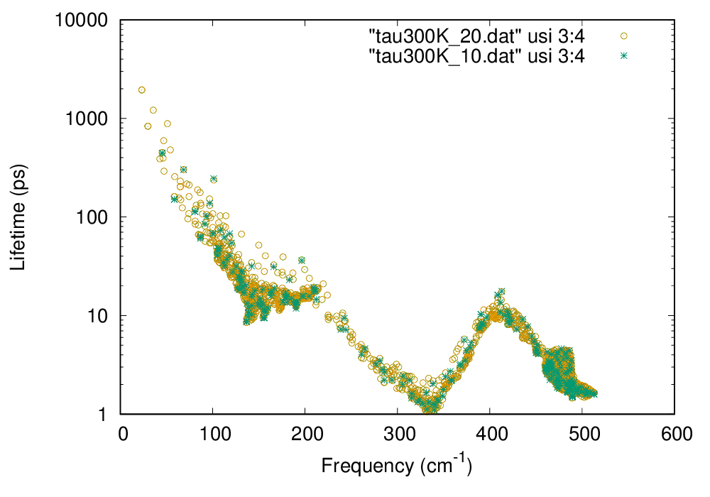
Phonon lifetime of Si at 300 K (click to enlarge)
In the above figure, phonon lifetimes calculated with \(20\times 20\times 20\ q\) points are also shown by open circles.
Cumulative thermal conductivity
Following the procedure below, you can obtain the cumulative thermal conductivity:
$ analyze_phonons.py --calc cumulative --temp 300 --length 10000:5 si222.result > cumulative_300K_10.dat
$ gnuplot
gnuplot> set logscale x
gnuplot> set xlabel "L (nm)"
gnuplot> set ylabel "Cumulative kappa (W/mK)"
gnuplot> plot "cumulative_300K_10.dat" using 1:2 w lp
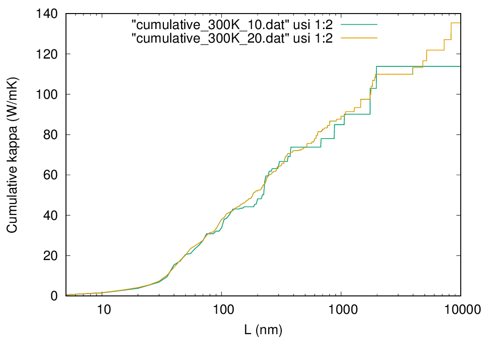
Cumulative thermal conductivity of Si at 300 K (click to enlarge)
To draw a smooth line, you have to use a denser \(q\) grid as shown in the figure by the orange line, which are obtained with \(20\times 20\times 20\ q\) points.
Thermal conductivity spectrum
To calculate the spectrum of thermal conductivity, modify the si_RTA.in as follows:
&general
  PREFIX = si222
  MODE = RTA
  FCSXML = si222_cubic.xml

  NKD = 1; KD = Si
  MASS = 28.0855

  EMIN = 0; EMAX = 550; DELTA_E = 1.0 # <-- frequency range
/

&cell
10.203
 0.0 0.5 0.5
 0.5 0.0 0.5
 0.5 0.5 0.0
/

&kpoint
 2
 10 10 10
/

&analysis
 KAPPA_SPEC = 1 # compute spectrum of kappa
/
The frequency range is specified with the EMIN, EMAX, and DELTA_E tags, and the KAPPA_SPEC = 1 is set in the &analysis field. Then, execute anphon again
$ anphon si_RTA.in > si_RTA2.log
After the calculation finishes, you can find the file si222.kl_spec which contains the spectra of thermal conductivity at various temperatures. You can plot the data at room temperature as follows:
$ awk '{if ($1 == 300.0) print $0}' si222.kl_spec > si222_300K_10.kl_spec
$ gnuplot
gnuplot> set xlabel "Frequency (cm^{-1})"
gnuplot> set ylabel "Spectrum of kappa (W/mK/cm^{-1})"
gnuplot> plot "si222_300K_10.kl_spec" using 2:3 w l lt 2 lw 2
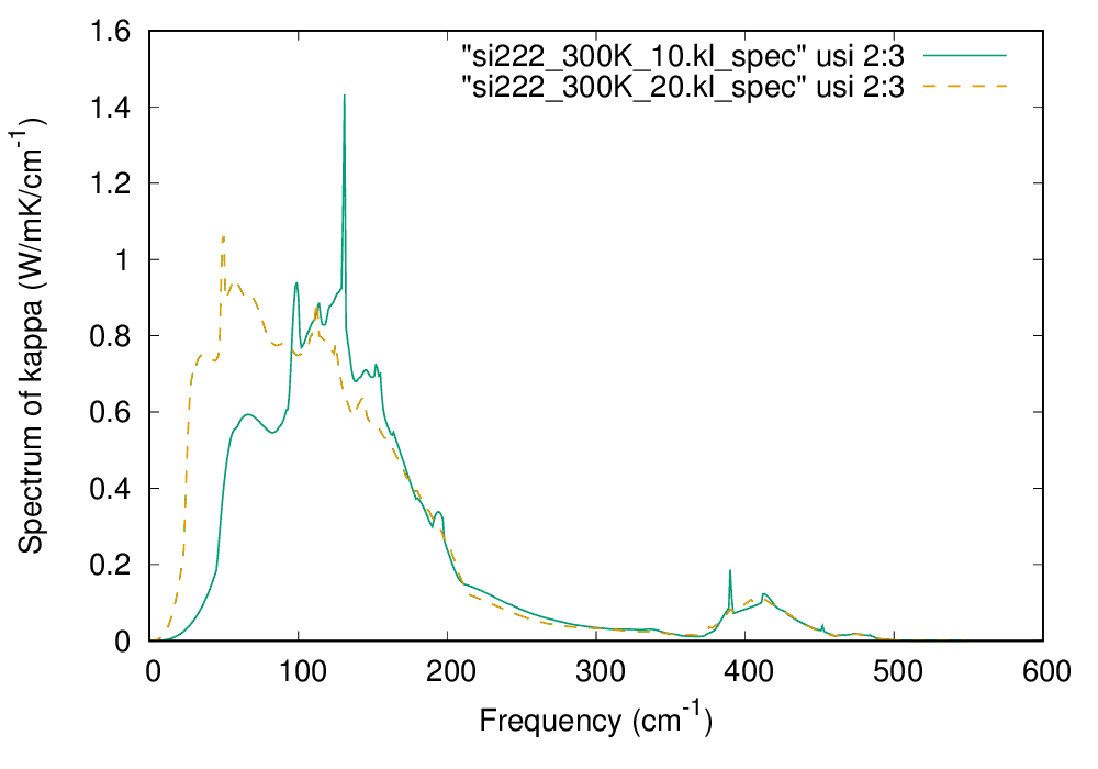
The spectrum of thermal conductivity of Si at 300 K (click to enlarge)
In the above figure, the computational result with \(20\times 20\times 20\ q\) points is also shown by the dashed line. From the figure, we can observe that low-energy phonons below 200 cm\(^{-1}\) account for more than 80% of the total thermal conductivity at 300 K.