7.5. BaTiO3 : Anharmonic interatomic force constants (IFCs)
This page explains how to calculate anharmonic interatomic force constants (IFCs) using ALAMODE, especially for strongly anharmonic materials. The target material is cubic BaTiO3, which exhibits a strong lattice anharmonicity.
The example input files are provided in example/BaTiO3/anharm_IFCs.
Let’s move to the example directory.
$ cd ${ALAMODE_ROOT}/example/BaTiO3/anharm_IFCs
1. Generate the randomly displaced supercells
Note
There is a more efficient way to generate supercells with random displacements for weakly anharmonic materials or materials without imaginary harmonic frequencies. Please see Tutorial 7.6 for details.
We use the ab initio molecular dynamics (AIMD) calculations to generate the supercells with random displacements.
The example VASP inputs are provided in example/BaTiO3/anharm_IFCs/1_vasp_md. Prepare the POTCAR file by yourself and run the AIMD calculation to obtain vasprun.xml (You can skip this part because vasprun.xml is provided in 1_vasp_md/reference).
Next, we generate the supercells with random atomic displacements from the AIMD trajectory. First, we move to the 1_configurations directory and copy vasprun.xml
$ cd 1_configurations
$ cp ../1_vasp_md/vasprun.xml ./ # If you have performed the AIMD calculation
$ cp ../1_vasp_md/reference/vasprun.xml ./ # If you skip the AIMD and use the reference result
POSCAR_ref_supercell is the structure of the reference supercell for which we want to calculate the IFCs.
$ python3 ${ALAMODE_ROOT}/tools/displace.py --VASP POSCAR_ref_supercell -md vasprun.xml -e 1001:5000:50 --random --mag 0.04 --prefix disp_aimd+random_
Here, the option -e 1001:5000:50 means that we sample from the 1001-th snapshot to the 5000-th snapshot with the sampling step of 50 time-steps.
Thus, 80 configurations are generated in this case.
The option --random --mag 0.04 adds random displacements of 0.04 Å to each atom in the extracted snapshots to reduce correlations between successive snapshots.
Note
We may use a less strict convergence criterion in the AIMD calculation because its purpose is just to generate the random structure, and the atomic forces obtained in AIMD are not directly used to calculate the IFCs. In fact, we use the following parameters, which are different from the subsequent calculation of the displacement-force data.
ENCUT = 400, EDIFF = 1.0E-6
2x2x2 kmesh
The temperature in the AIMD calculation is chosen so that the generated trajectory widely samples the low-energy landscape of the potential energy surface. We choose 300 K in this case, which is comparable to or lower than the structural transition temperatures of the target material.
Note
The number of random configurations should be chosen so that the generated set of IFCs converges with respect to it. Ideally, we should check the convergence of the calculated physical quantities by changing the number of random configurations from which we extract the anharmonic IFCs.
It depends on the problems, but a rule of thumb tells us that 100~1000 configurations will do for the calculation of cubic and quartic IFCs. We can reduce the number of configurations if we calculate only the cubic IFCs.
2. Generate the displacement-force data
We calculate the atomic forces for each random configuration generated in the previous step.
The other VASP input files (INCAR and KPOINTS) are provided in example/BaTiO3/anharm_IFCs/2_vasp_dfset. After running the VASP calculations, collect the resultant vasprun.xml of each calculation in example/BaTiO3/anharm_IFCs/2_vasp_dfset.
If you want to skip the VASP calculations, please copy or move the 80 vasprun.xml files provided in 2_vasp_dfset/reference to 2_vasp_dfset.
Generate the displacement-force data with the command
$ cd ${ALAMODE_ROOT}/example/BaTiO3/anharm_IFCs/2_vasp_dfset
$ cp ../1_configurations/POSCAR_ref_supercell ./
$ python3 ${ALAMODE_ROOT}/tools/extract.py --VASP=POSCAR_ref_supercell vasprun*.xml > DFSET_AIMD_random
The generated DFSET_AIMD_random stores the atomic displacements and the atomic forces in each configuration, from which we can calculate the anharmonic IFCs.
3. Cross validation (CV)
We assume that the harmonic force constants are already calculated. Please use the method explained in Tutorial 7.1 for the calculation of harmonic IFCs.
In the cross validation, we determine the optimal amplitude of regularization (\(\alpha\)) in the elastic-net or adaptive lasso. Please see the documentation for the notation and the theoretical background.
You can run the CV calculation with the following commands.
$ cd ${ALAMODE_ROOT}/example/BaTiO3/3_cv
$ ${ALAMODE_ROOT}/alm/alm BTO_alm_cv.in > BTO_alm_cv.log
In BTO_alm_cv.in, FC2XML = ../cBTO222_harmonic.xml means that we fix the harmonic IFCs with the values in the given file.
This is because we would like to capture the stability or the curvature of the potential energy surface at the reference structure accurately.
Note
With NBODY = 2 3 3, we restrict the quartic IFCs to up-to-three-body terms.
This treatment reduces the computational cost and makes the fitting more robust by reducing the number of degrees of freedom.
Although the best choice of NBODY-tag will depend on the materials and on the number of your displacement-force data,
we recommend restricting the quartic IFCs to up-to-three-body terms and the higher order IFCs to up-to-two-body terms
since the higher-order IFCs will be more localized in space.
Plotting the generated cBTO222.cvscore with
$ gnuplot cv_plot.plt
we get the following plot.
Note that you need to set STOP_CRITERION = 30 in &optimize-field to get exactly the same plot.
Otherwise, the calculation is stopped before calculations with small \(\alpha\) are performed to save the computational cost.
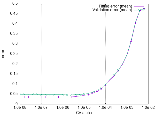
The result of the CV calculation for BaTiO3.
We can see that the CV score takes a minimum at the optimal \(\alpha\), which can be read from the last line of cBTO222.cvscore.
# Minimum CVSCORE at alpha = 2.51189e-06
4. Calculation of IFCs
Finally, we calculate the IFCs of BaTiO3 in example/BaTiO3/anharm_IFCs/4_optimize.
$ cd ${ALAMODE_ROOT}/example/BaTiO3/4_optimize
To prepare the input file, we copy the input of CV and set L1_ALPHA with the optimal value
by adding the new line in &optimize-field.
L1_ALPHA = 2.51189e-06
Also, change CV=4 in &optimize-field to
CV = 0 # switch off CV
You can also use a smaller value for CONV_TOL to get a more accurate result.
With the input file prepared, run the calculation with
$ ${ALAMODE_ROOT}/alm/alm BTO_alm_opt.in > BTO_alm_opt.log
The calculated IFCs are written out in cBTO222.fcs and cBTO222.xml.
Checking BTO_alm_opt.log, we can see that the fitting is successful with a small residual error.
RESIDUAL (%): 3.91121