7.8. ZnO : A QHA-based structural optimization example

This page explains how to calculate crystal structures at finite temperatures (\(T\)) based on the quasiharmonic approximation (QHA).

Let’s move to the example directory

$ cd ${ALAMODE_ROOT}/example/ZnO/qha_relax

1. Prepare force constants

This tutorial assumes that the harmonic and anharmonic force constants are already calculated up to fourth order. Here, please unzip all the XML files in example/ZnO/qha_relax and example/ZnO/qha_relax/strain_IFC before running the calculation.

Note

We use the harmonic IFCs calculated in the \(4\times 4\times 2\) supercell and the anharmonic IFCs calculated in the \(3\times 3\times 2\) supercell due to the high computational cost of the DFT calculations for the anharmonic IFCs. This treatment is justified because the higher-order IFCs tend to be more localized in real space.

2. Prepare the additional input files.

We need to calculate the elastic constants, the strain-force coupling, and the strain-harmonic-IFC coupling to calculate the \(T\)-dependence of the shape of the unit cell. These input files must be placed in the directory named as the value of STRAIN_IFC_DIR-tag, specified in &relax-field in the input file of anphon.

• The second-order elastic constants (SOEC) and the third-order elastic constants (TOEC) need to be calculated by yourself. The name of the input file must be elastic_constants.in. The format of elastic_constants.in is as follows.

  SOEC
  V_cell * C_xx,xx
  V_cell * C_xx,xy
  V_cell * C_xx,xz
  ...
  V_cell * C_zz,zz
  TOEC
  V_cell * C_xx,xx,xx
  V_cell * C_xx,xx,xy
  ...
  V_cell * C_zz,zz,zz
  

  \(V_{cell}\) is the shape of the unit cell and \(C_{\mu_1 \nu_1, \mu_2 \nu_2} = \frac{1}{V}\frac{\partial U}{\partial u_{\mu_1 \nu_1} \partial u_{\mu_2 \nu_2}}\), \(C_{\mu_1 \nu_1, \mu_2 \nu_2, \mu_3 \nu_3} = \frac{1}{V}\frac{\partial U}{\partial u_{\mu_1 \nu_1} \partial u_{\mu_2 \nu_2} \partial u_{\mu_3 \nu_3}}\) are the second-order and third-order elastic constants. The values in elastic_constants.in should be in Rydberg unit.

• The strain-force coupling can be calculated using the strainIFCcoupling code.

  Suppose the strain-force coupling is zero, i.e., the atomic force is zero when we apply finite strain with fixed fractional atomic coordinates. In that case you can set RENORM_2TO1ST=0 and omit the corresponding input file. To use RENORM_2TO1ST=1, we need to impose rotational invariance on the IFCs (See Appendix C of the original paper for the proof), which is not recommended because it usually worsens the fitting error.

  The name of the input file of the strain-force coupling must be strain_force.in.

  In this tutorial, the following block of the input file means that if we apply the strain \(u_{xx}= 0.005\), the atomic force that acts on the first atom is \((f_x, f_y, f_z) = (0.000000, -0.034812, -0.022224)\) [Ry/Bohr], e.t.c.

  xx 0.005 1.0
  0.000000  -0.034812  -0.022224
  0.000000  0.034812  -0.022224
  0.000000  -0.039854  0.022224
  0.000000  0.039854  0.022224
  

  The meaning of the weight 1.0 is similar to that in the next paragraph.

  Note that if we use the strainIFCcoupling code, we can obtain a set of input files that follows this format.

• The strain-harmonic-IFC coupling can be calculated using the strainIFCcoupling code. The input files are strain_harmonic.in and the related XML files.

  For example,

  xx 0.005 1.0 ZnO442_harmonic_xx_0005.xml
  

  in strain_harmonic.in means that ZnO442_harmonic_xx_0005.xml is the XML file of the harmonic IFCs with the strain \(u_{xx} = 0.005\). The weight is 1.0 in this case because we use the one-sided difference to calculate

  \(\frac{\partial \widetilde{\Phi}_{\mu\mu'}(0\alpha,R'\alpha')}{\partial u_{xx}} \simeq \frac{\widetilde{\Phi}(u_{xx} = 0.005) - \widetilde{\Phi}(u_{\mu \nu} = 0.0)}{0.005}\).

  If you use the central difference method

  \(\frac{\partial \widetilde{\Phi}_{\mu\mu'}(0\alpha,R'\alpha')}{\partial u_{xx}} \simeq \frac{\widetilde{\Phi}(u_{xx} = 0.005) - \widetilde{\Phi}(u_{xx} = -0.005)}{0.005\times2}\)

  \(= 0.5\times \frac{\widetilde{\Phi}(u_{xx} = 0.005) - \widetilde{\Phi}(u_{\mu \nu} = 0.0)}{0.005} + 0.5\times \frac{\widetilde{\Phi}(u_{xx} = -0.005) - \widetilde{\Phi}(u_{\mu \nu} = 0.0)}{-0.005}\),

  the corresponding strain_harmonic.in would be like

  xx 0.005 0.5 ZnO442_harmonic_xx_0005.xml
  xx 0.005 0.5 ZnO442_harmonic_xx_minus_0005.xml
  

  with respective weights of 0.5 (ZnO442_harmonic_xx_minus_0005.xml is not provided in this tutorial).

  For the off-diagonal strain,

  yz 0.005 1.0 ZnO442_harmonic_yz_00025.xml
  

  means that ZnO442_harmonic_yz_00025.xml is the set of harmonic IFCs with \(u_{yz} = u_{zy} = 0.005/2 = 0.0025\).

  Note that if you use the strainIFCcoupling code, you can obtain a set of input files that follows this format.

3. Prepare the input file.

The input file for the anphon calculation is ZnO_qha_thermo.in.

Note

We set KMESH_QHA = 4 4 2 to save the computational cost. In addition, the convergence threshold of the structural optimization (COORD_CONV_TOL = 1.0e-5 and CELL_CONV_TOL = 1.0e-5) may not be small enough if you want to calculate the thermal expansion coefficient \(\alpha(T) = \frac{1}{V}\frac{\partial V}{\partial T}\) by finite-difference method with a small temperature difference.

These parameters should be chosen carefully to obtain accurate calculation results.

Run the calculation with

$ ${ALAMODE_ROOT}/anphon/anphon ZnO_qha_thermo.in > ZnO_qha_thermo.log

4. Analyze the calculation results.

We can plot the \(T\)-dependence of the thermal strain, which is written in ZnO_qha.umn_tensor, with

$ gnuplot plot.plt

to obtain the followin figure.

We can see that the thermal expansion is negative at low temperatures, and it turns positive at high temperatures. The pace of expansion of the \(a\)-axis is faster than that of the \(c\)-axis, which agrees with the result in the paper.

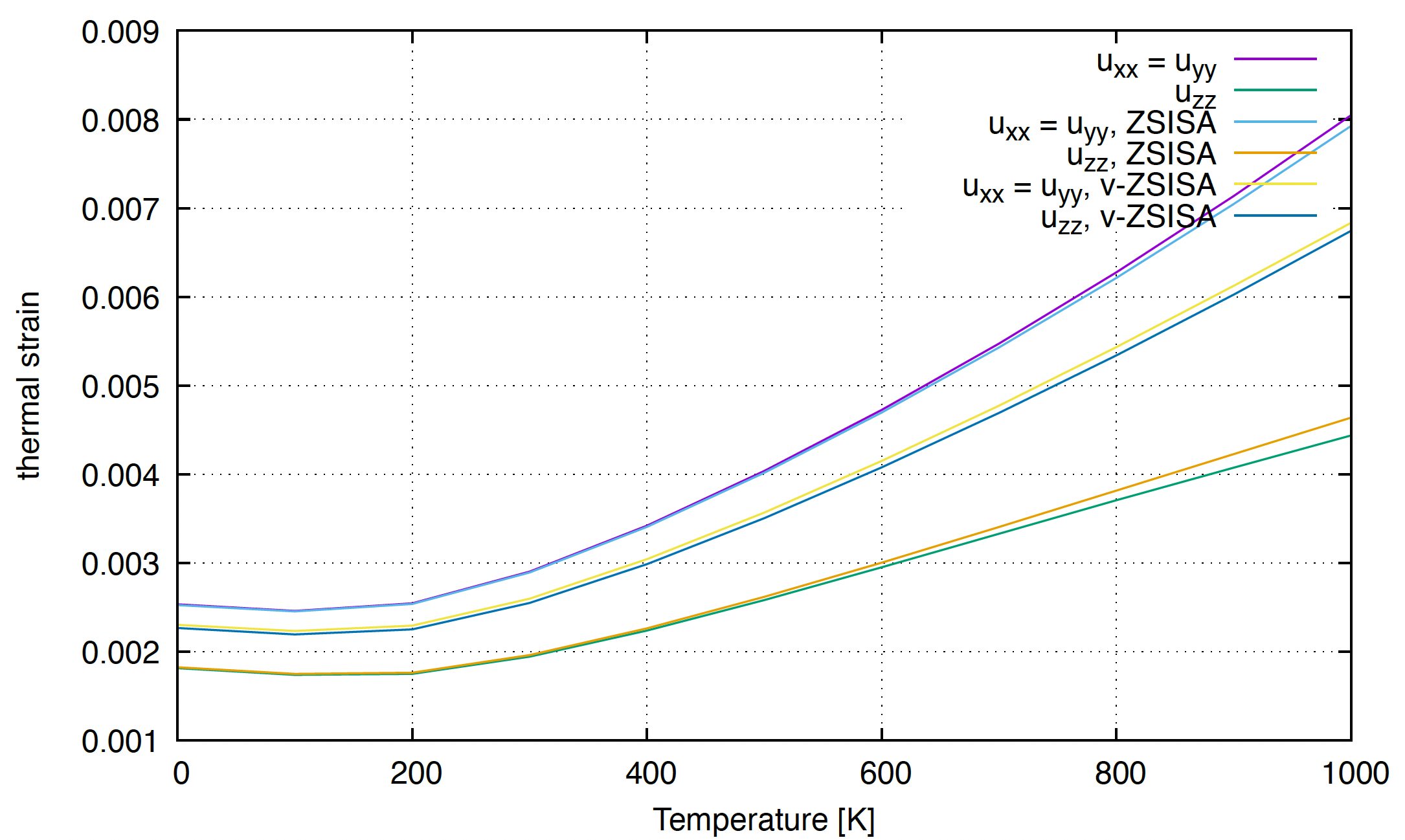
The temperature-dependence of the thermal strain of ZnO. In this wurtzite case, \(u_{xx} = u_{yy} = a(T)/a(T=0)-1.0\), \(u_{zz} = c(T)/c(T=0)-1.0\), where \(a(T)\) and \(c(T)\) are the \(T\)-dependent lengths of the \(a\) and \(c\)-axis respectively.

The ZSISA (zero static internal stress approximation) and the v-ZSISA (volumetric ZSISA) are approximate optimization schemes often used in QHA calculations. The definition and the accuracy of these methods are discussed in our original paper.

ZSISA and v-ZSISA calculations can be performed by changing QHA_SCHEME-tag in &qha-field. We can see that ZSISA accurately reproduces the \(T\)-dependence of the unit cell shape. v-ZSISA underestimates the anisotropy of the thermal expansion, while it gives a good estimation of the \(T\)-dependence of the volume of the unit cell, which is consistent with the general theorem shown in the paper.

We can also calculate the \(T\)-induced change of the electric polarization by

\(P_{\mu}(T) - P_{\mu}(T=0) =\frac{1}{V_{cell}} \sum_{\alpha \nu} Z^*_{\alpha \mu \nu} u^{(0)}_{\alpha \nu}+\sum_{\mu_1 \nu_1}d_{\mu, \mu_1 \nu_1} u_{\mu_1 \nu_1},\)

where \(Z^*_{\alpha \mu \nu}\) are the Born effective charges and \(d_{\mu, \mu_1 \nu_1}\) are the piezoelectric tensors, which can be calcualted using DFPT in the reference structure. The \(T\)-dependent atomic displacements \(u^{(0)}_{\alpha \nu}\) and the strain tensor \(u_{\mu_1 \nu_1}\) are written in ZnO_qha.atom_disp and ZnO_qha.umn_tensor respectively.